本文深入剖析Transformer的核心创新——Self-Attention机制,通过数学推导、代码实现和可视化,全面讲解Query/Key/Value概念、Scaled Dot-Product Attention原理以及Multi-Head Attention实现细节。
graph LR
    A[RNN/LSTM] --> B[顺序处理]
    B --> C[无法并行]
    C --> D[长程依赖衰减]
    D --> E[梯度消失/爆炸]
1.2 Self-Attention核心思想
import torch
import torch.nn as nn
import numpy as np
import matplotlib.pyplot as plt
# 输入序列 (batch_size=1, seq_length=4, embedding_dim=8)
x = torch.tensor([[
[1.0, 0.5, 0.8, 2.0, 0.1, 1.5, 0.3, 1.2],
[0.7, 1.2, 0.4, 1.8, 0.9, 0.6, 1.1, 0.2],
[1.3, 0.3, 1.7, 0.6, 1.4, 0.8, 0.5, 1.9],
[0.2, 1.5, 1.1, 0.7, 0.3, 1.8, 1.6, 0.4]
]])
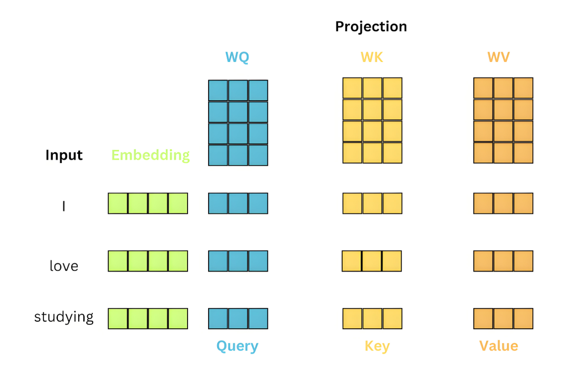
print("输入序列形状:", x.shape)Self-Attention三大核心向量:
Query (Q):当前关注的词向量
Key (K):用于被查询的标识向量
Value (V):实际传递信息的向量
class SelfAttention(nn.Module):
    def __init__(self, embed_size):
        super().__init__()
        self.embed_size = embed_size
        # 线性变换层
        self.Wq = nn.Linear(embed_size, embed_size)
        self.Wk = nn.Linear(embed_size, embed_size)
        self.Wv = nn.Linear(embed_size, embed_size)

    def forward(self, x):
        Q = self.Wq(x)  # Query
        K = self.Wk(x)  # Key
        V = self.Wv(x)  # Value
        return Q, K, V
# 生成Q,K,V
attention = SelfAttention(embed_size=8)
Q, K, V = attention(x)
print("Query形状:", Q.shape)
print("Key形状:", K.shape)
print("Value形状:", V.shape)
Self-Attention核心优势:
全局依赖:直接捕获任意位置间的关系
并行计算:所有位置同时计算注意力
长程建模:无距离衰减的信息传递
可解释性:注意力权重可视化决策依据
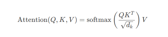
计算步骤分解:
相似度计算:$QK^T$(查询与键的点积)
缩放处理:除以$\sqrt{d_k}$(防止梯度消失)
权重归一化:softmax函数
加权求和:乘以Value向量
def scaled_dot_product_attention(Q, K, V):
    # Step 1: 计算Q和K的点积
    matmul_qk = torch.matmul(Q, K.transpose(-2, -1))

    # Step 2: 缩放处理
    d_k = K.size(-1)
    scaled_attention_logits = matmul_qk / torch.sqrt(torch.tensor(d_k, dtype=torch.float32))

    # Step 3: softmax归一化
    attention_weights = torch.softmax(scaled_attention_logits, dim=-1)

    # Step 4: 加权求和
    output = torch.matmul(attention_weights, V)

    return output, attention_weights
# 计算注意力
output, attn_weights = scaled_dot_product_attention(Q, K, V)
print("注意力输出形状:", output.shape)
print("注意力权重形状:", attn_weights.shape)# 可视化注意力权重
plt.figure(figsize=(10, 8))
plt.imshow(attn_weights.detach().squeeze().numpy(), cmap='viridis')
plt.title('Self-Attention权重矩阵')
plt.xlabel('Key位置')
plt.ylabel('Query位置')
plt.colorbar()
plt.xticks(range(4), ['词1', '词2', '词3', '词4'])
plt.yticks(range(4), ['词1', '词2', '词3', '词4'])
# 添加权重值
for i in range(attn_weights.shape[-2]):
for j in range(attn_weights.shape[-1]):
plt.text(j, i, f"{attn_weights[0,i,j].item():.2f}",
ha="center", va="center", color="w")
plt.show()缩放因子$\sqrt{d_k}$的数学意义:
假设$q$和$k$是独立随机变量,均值为0,方差为1
则点积$q \cdot k = \sum_{i=1}^{d_k} q_i k_i$的:
均值:$E[q \cdot k] = 0$
方差:$\text{Var}(q \cdot k) = d_k$
缩放后方差变为1,保持梯度稳定性:

graph LR
    A[输入向量] --> B[线性变换]
    B --> C1[头1 QKV]
    B --> C2[头2 QKV]
    B --> C3[头n QKV]
    C1 --> D1[Scaled Dot-Attention]
    C2 --> D2[Scaled Dot-Attention]
    C3 --> Dn[Scaled Dot-Attention]
    D1 --> E[拼接输出]
    D2 --> E
    Dn --> E
    E --> F[线性变换]
    F --> G[最终输出]
class MultiHeadAttention(nn.Module):
    def __init__(self, embed_size, num_heads):
        super().__init__()
        self.embed_size = embed_size
        self.num_heads = num_heads
        self.head_dim = embed_size // num_heads

        assert self.head_dim * num_heads == embed_size, "嵌入维度必须是头数的整数倍"

        # 线性变换层
        self.Wq = nn.Linear(embed_size, embed_size)
        self.Wk = nn.Linear(embed_size, embed_size)
        self.Wv = nn.Linear(embed_size, embed_size)
        self.fc_out = nn.Linear(embed_size, embed_size)

    def split_heads(self, x):
        """将嵌入维度分割为多个头"""
        batch_size, seq_length, _ = x.size()
        return x.view(batch_size, seq_length, self.num_heads, self.head_dim).transpose(1, 2)

    def forward(self, Q, K, V, mask=None):
        batch_size = Q.size(0)

        # 线性变换
        Q = self.Wq(Q)
        K = self.Wk(K)
        V = self.Wv(V)

        # 分割多头
        Q = self.split_heads(Q)  # (batch_size, num_heads, seq_len, head_dim)
        K = self.split_heads(K)
        V = self.split_heads(V)

        # 计算缩放点积注意力
        attn_output, attn_weights = scaled_dot_product_attention(Q, K, V)

        # 拼接多头输出
        attn_output = attn_output.transpose(1, 2).contiguous().view(
            batch_size, -1, self.embed_size)

        # 最终线性变换
        output = self.fc_out(attn_output)

        return output, attn_weights
# 测试多头注意力
embed_size = 8
num_heads = 2
multihead_attn = MultiHeadAttention(embed_size, num_heads)
output, attn_weights = multihead_attn(x, x, x)
print("多头注意力输出形状:", output.shape)
print("多头注意力权重形状:", attn_weights.shape) # (batch_size, num_heads, seq_len, seq_len)# 可视化不同头的注意力权重
fig, axes = plt.subplots(1, num_heads, figsize=(15, 5))
for i in range(num_heads):
ax = axes[i]
head_weights = attn_weights[0, i].detach().numpy()
im = ax.imshow(head_weights, cmap='viridis')
ax.set_title(f'头 {i+1} 注意力权重')
ax.set_xlabel('Key位置')
ax.set_ylabel('Query位置')
fig.colorbar(im, ax=ax)
# 添加权重值
for row in range(head_weights.shape[0]):
for col in range(head_weights.shape[1]):
ax.text(col, row, f"{head_weights[row, col]:.2f}",
ha="center", va="center", color="w", fontsize=8)
plt.tight_layout()
plt.show()多头注意力的优势:
多视角建模:每个头关注不同特征空间
并行计算:多个头可同时独立计算
表征能力增强:组合不同子空间信息
可解释性提升:不同头可学习不同关系
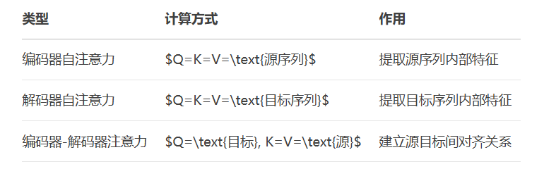
编码器自注意力:源序列内部关系
encoder_self_attn = MultiHeadAttention(embed_size, num_heads)
encoder_output, _ = encoder_self_attn(src, src, src)
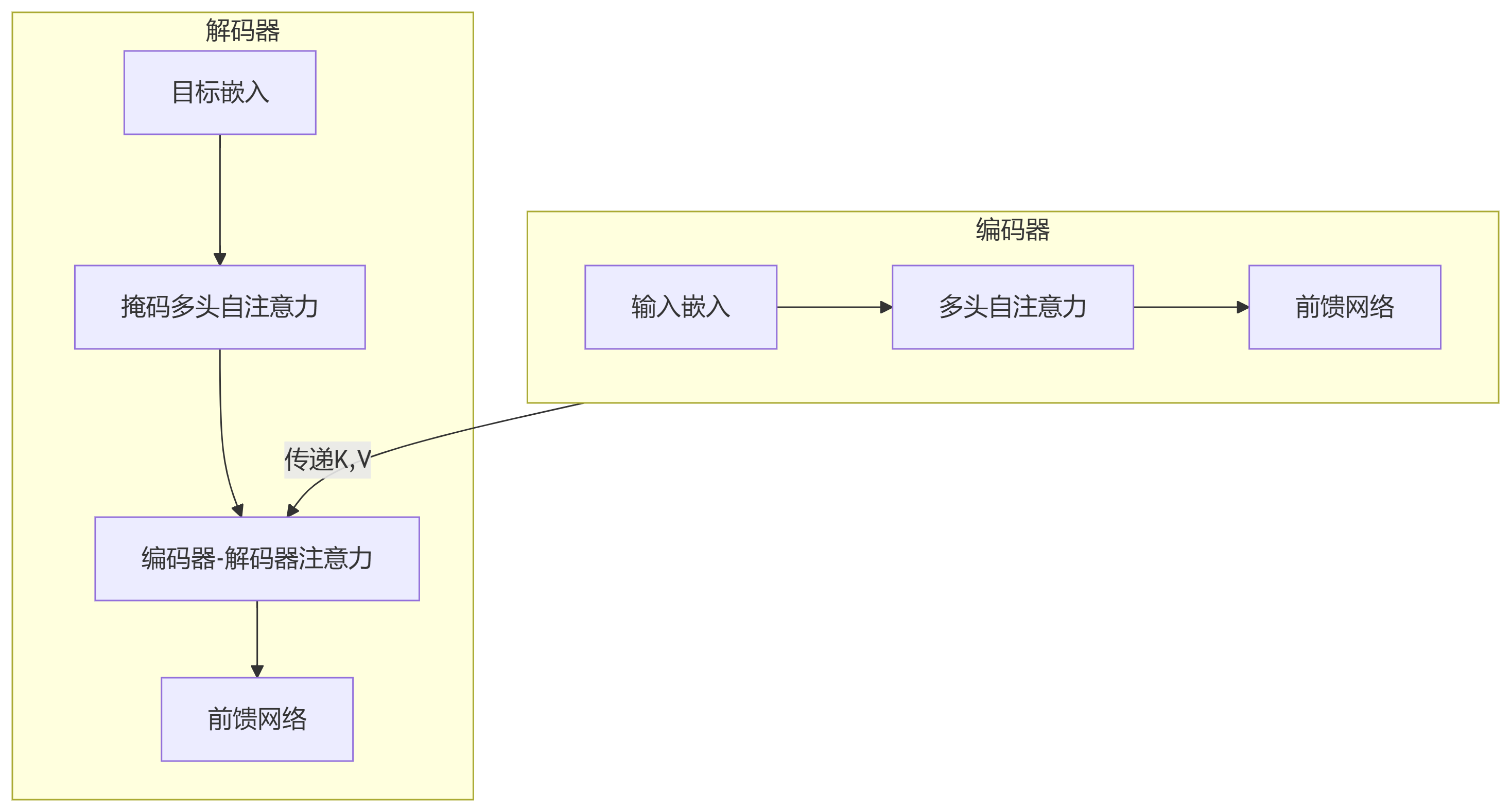
解码器自注意力:目标序列内部关系(带掩码)
# 创建下三角掩码
def create_mask(size):
    mask = torch.tril(torch.ones(size, size))
    return mask.masked_fill(mask == 0, float('-inf'))
mask = create_mask(tgt.size(1))
decoder_self_attn = MultiHeadAttention(embed_size, num_heads)
decoder_output, _ = decoder_self_attn(tgt, tgt, tgt, mask)编码器-解码器注意力:源序列与目标序列间关系
cross_attn = MultiHeadAttention(embed_size, num_heads)
cross_output, _ = cross_attn(decoder_output, encoder_output, encoder_output)
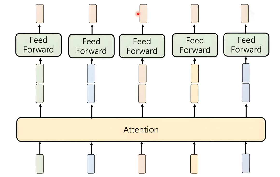
4.3 完整Transformer层实现
class TransformerBlock(nn.Module):
    """完整的Transformer编码器层"""
    def __init__(self, embed_size, num_heads, ff_dim, dropout=0.1):
        super().__init__()
        # 多头注意力
        self.attention = MultiHeadAttention(embed_size, num_heads)
        # 前馈网络
        self.feed_forward = nn.Sequential(
            nn.Linear(embed_size, ff_dim),
            nn.ReLU(),
            nn.Linear(ff_dim, embed_size)
        )
        # 归一化层
        self.norm1 = nn.LayerNorm(embed_size)
        self.norm2 = nn.LayerNorm(embed_size)
        # Dropout
        self.dropout = nn.Dropout(dropout)

    def forward(self, x):
        # 残差连接1
        attn_output, _ = self.attention(x, x, x)
        x = self.norm1(x + self.dropout(attn_output))

        # 残差连接2
        ff_output = self.feed_forward(x)
        x = self.norm2(x + self.dropout(ff_output))

        return x
# 测试Transformer层
transformer_block = TransformerBlock(
    embed_size=8,
    num_heads=2,
    ff_dim=32
)
output = transformer_block(x)
print("Transformer层输出形状:", output.shape)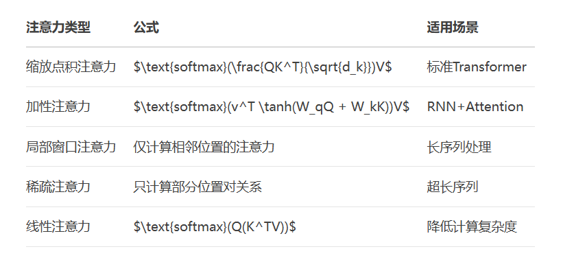
5.2 自注意力与卷积的融合
class ConvAttention(nn.Module):
    """卷积增强的自注意力"""
    def __init__(self, embed_size, num_heads, kernel_size=3):
        super().__init__()
        self.attention = MultiHeadAttention(embed_size, num_heads)
        self.conv = nn.Conv1d(
            in_channels=embed_size,
            out_channels=embed_size,
            kernel_size=kernel_size,
            padding=kernel_size//2
        )
        self.norm = nn.LayerNorm(embed_size)

    def forward(self, x):
        # 自注意力路径
        attn_out, _ = self.attention(x, x, x)

        # 卷积路径 (需要调整维度)
        conv_out = self.conv(x.transpose(1, 2)).transpose(1, 2)

        # 融合并归一化
        combined = attn_out + conv_out
        return self.norm(combined)
# 测试卷积注意力
conv_attn = ConvAttention(embed_size=8, num_heads=2)
output = conv_attn(x)
print("卷积注意力输出形状:", output.shape)class EfficientAttention(nn.Module):
"""线性复杂度的注意力机制"""
def __init__(self, embed_size):
super().__init__()
self.embed_size = embed_size
# 特征变换
self.to_query = nn.Linear(embed_size, embed_size)
self.to_key = nn.Linear(embed_size, embed_size)
self.to_value = nn.Linear(embed_size, embed_size)
def forward(self, x):
Q = self.to_query(x)
K = self.to_key(x)
V = self.to_value(x)
# 高效计算 (避免显式计算QK^T)
K = K.softmax(dim=1)
context = torch.einsum('bnd,bne->bde', K, V)
output = torch.einsum('bnd,bde->bne', Q, context)
return output
# 测试高效注意力
eff_attn = EfficientAttention(embed_size=8)
output = eff_attn(x)
print("高效注意力输出形状:", output.shape)from torchtext.datasets import IMDB
from torchtext.data import get_tokenizer
from torchtext.vocab import build_vocab_from_iterator
# 加载IMDB数据集
train_iter = IMDB(split='train')
tokenizer = get_tokenizer('basic_english')
# 构建词汇表
def yield_tokens(data_iter):
for _, text in data_iter:
yield tokenizer(text)
vocab = build_vocab_from_iterator(yield_tokens(train_iter), specials=['<unk>', '<pad>'])
vocab.set_default_index(vocab['<unk>'])
# 文本转张量
def text_pipeline(text):
return vocab(tokenizer(text))
# 创建批次处理函数
def collate_batch(batch, max_len=512):
label_list, text_list = [], []
for label, text in batch:
label_list.append(1 if label=='pos' else 0)
processed_text = text_pipeline(text)[:max_len]
processed_text += [vocab['<pad>']] * (max_len - len(processed_text))
text_list.append(processed_text)
return torch.tensor(label_list), torch.tensor(text_list)
# 创建数据加载器
from torch.utils.data import DataLoader
train_loader = DataLoader(
list(IMDB(split='train')),
batch_size=32,
collate_fn=collate_batch
)class AttentionClassifier(nn.Module): def __init__(self, vocab_size, embed_dim, num_heads, hidden_dim, num_classes): super().__init__() # 嵌入层 self.embedding = nn.Embedding(vocab_size, embed_dim) # 位置编码 self.pos_encoding = nn.Parameter(torch.randn(1, 512, embed_dim)) # 自注意力层 self.attention = MultiHeadAttention(embed_dim, num_heads) # 分类器 self.classifier = nn.Sequential( nn.Linear(embed_dim, hidden_dim), nn.ReLU(), nn.Dropout(0.5), nn.Linear(hidden_dim, num_classes) ) def forward(self, x): # 嵌入层 x = self.embedding(x) # (batch, seq, embed_dim) # 添加位置编码 seq_len = x.size(1) x = x + self.pos_encoding[:, :seq_len, :] # 自注意力 attn_output, _ = self.attention(x, x, x) # 全局平均池化 pooled = attn_output.mean(dim=1) # 分类 return self.classifier(pooled) # 初始化模型 vocab_size = len(vocab) model = AttentionClassifier( vocab_size=vocab_size, embed_dim=128, num_heads=4, hidden_dim=256, num_classes=2 ) # 训练配置 criterion = nn.CrossEntropyLoss() optimizer = torch.optim.Adam(model.parameters(), lr=0.001)
# 训练循环
for epoch in range(5):
    total_loss = 0
    correct = 0
    total = 0

    for labels, texts in train_loader:
        optimizer.zero_grad()
        outputs = model(texts)
        loss = criterion(outputs, labels)
        loss.backward()
        optimizer.step()

        total_loss += loss.item()
        _, predicted = outputs.max(1)
        total += labels.size(0)
        correct += predicted.eq(labels).sum().item()

    accuracy = 100. * correct / total
    print(f"Epoch {epoch+1}, Loss: {total_loss/len(train_loader):.4f}, Acc: {accuracy:.2f}%")
# 可视化样本注意力
def visualize_attention(text):
    # 预处理文本
    tokens = tokenizer(text)
    indexed = [vocab[token] for token in tokens][:512]
    input_tensor = torch.tensor([indexed])

    # 获取模型输出和注意力权重
    model.eval()
    with torch.no_grad():
        embeddings = model.embedding(input_tensor)
        _, attn_weights = model.attention(embeddings, embeddings, embeddings)
        attn_weights = attn_weights.mean(dim=1)  # 平均多头

    # 可视化
    plt.figure(figsize=(12, 6))
    plt.imshow(attn_weights.squeeze().numpy(), cmap='viridis')
    plt.title('文本注意力权重')
    plt.xlabel('Key位置')
    plt.ylabel('Query位置')
    plt.xticks(range(len(tokens)), tokens, rotation=90)
    plt.yticks(range(len(tokens)), tokens)
    plt.colorbar()
    plt.tight_layout()
    plt.show()
# 测试样例
sample_text = "This movie is absolutely fantastic and captivating from start to finish"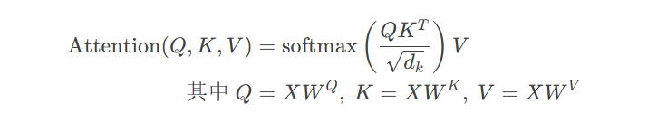
visualize_attention(sample_text)Self-Attention核心公式:
Multi-Head Attention处理流程:
flowchart LR
    A[输入] --> B[线性变换]
    B --> C[分割多头]
    C --> D[Scaled Dot-Product]
    D --> E[拼接输出]
    E --> F[线性变换]
    F --> G[输出]
Transformer中注意力的三种应用:
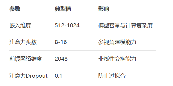
注意力机制超参数选择:
掌握Self-Attention机制是理解现代大模型的基础,通过本文的数学推导和代码实践,你已经具备了实现和优化注意力模型的核心能力!更多AI大模型应用开发学习视频内容和资料,尽在聚客AI学院。