本文全面剖析RNN核心原理,深入讲解梯度消失/爆炸问题,并通过LSTM/GRU结构实现解决方案,提供时间序列预测和文本生成完整代码实现。
import torch
import torch.nn as nn
import numpy as np
import matplotlib.pyplot as plt
# 手动实现RNN单元
class SimpleRNNCell:
    def __init__(self, input_size, hidden_size):
        # 权重初始化
        self.W_xh = torch.randn(input_size, hidden_size) * 0.01
        self.W_hh = torch.randn(hidden_size, hidden_size) * 0.01
        self.b_h = torch.zeros(1, hidden_size)

    def forward(self, x, h_prev):
        """
        x: 当前输入 (1, input_size)
        h_prev: 前一刻隐藏状态 (1, hidden_size)
        """
        # RNN核心计算
        h_next = torch.tanh(torch.mm(x, self.W_xh) +
                           torch.mm(h_prev, self.W_hh) +
                           self.b_h)
        return h_next
# 示例:处理序列数据
input_size = 3
hidden_size = 4
seq_length = 5
# 创建RNN单元
rnn_cell = SimpleRNNCell(input_size, hidden_size)
# 初始化隐藏状态
h = torch.zeros(1, hidden_size)
# 模拟输入序列 (5个时间步,每个时间步3维向量)
inputs = [torch.randn(1, input_size) for _ in range(seq_length)]
# 循环处理序列
hidden_states = []
for t in range(seq_length):
    h = rnn_cell.forward(inputs[t], h)
    hidden_states.append(h.detach().numpy())
    print(f"时间步 {t+1}, 隐藏状态: {h}")
# 可视化隐藏状态变化
plt.figure(figsize=(10, 6))
for i in range(hidden_size):
    plt.plot(range(1, seq_length+1), [h[0,i] for h in hidden_states],
             label=f'隐藏单元 {i+1}')
plt.title('RNN隐藏状态随时间变化')
plt.xlabel('时间步')
plt.ylabel('隐藏状态值')
plt.legend()
plt.grid(True)
plt.show()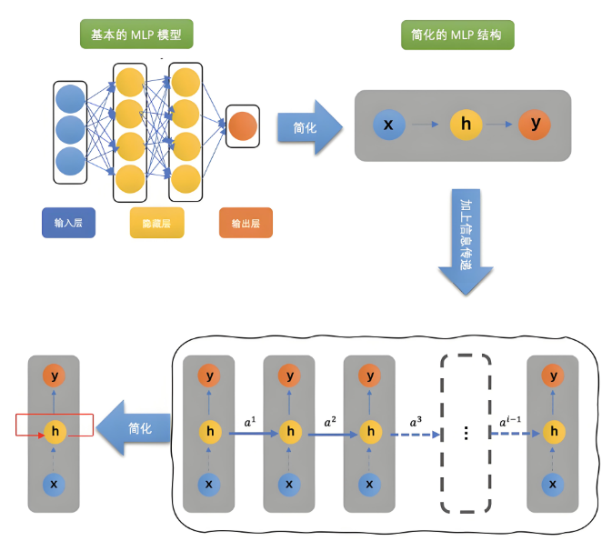
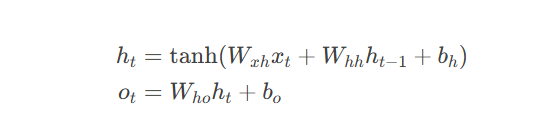
RNN数学原理:
RNN核心特点:
时间展开:在不同时间步共享相同权重
隐藏状态:传递序列历史信息
参数共享:显著减少参数量
# 使用PyTorch内置RNN
rnn = nn.RNN(input_size=3, hidden_size=4, num_layers=1, batch_first=True)
# 输入数据格式: (batch_size, seq_length, input_size)
inputs = torch.randn(1, 5, 3)  # 批量1, 序列长度5, 输入维度3
h0 = torch.zeros(1, 1, 4)      # 初始隐藏状态 (num_layers, batch_size, hidden_size)
# 前向传播
output, hn = rnn(inputs, h0)
print("输出形状:", output.shape)  # (1, 5, 4)
print("最终隐藏状态形状:", hn.shape) # (1, 1, 4)# 模拟梯度消失
def simulate_vanishing_grad(seq_length=20, num_runs=100):
# 初始化权重
W = torch.randn(1, 1) * 0.8 # |W| < 1
grad_history = []
for _ in range(num_runs):
# 初始化梯度
grad = 1.0
# 反向传播模拟
for t in range(seq_length):
grad = grad * W.item()
grad_history.append(grad)
return grad_history
# 模拟梯度爆炸
def simulate_exploding_grad(seq_length=20, num_runs=100):
# 初始化权重
W = torch.randn(1, 1) * 1.2 # |W| > 1
grad_history = []
for _ in range(num_runs):
# 初始化梯度
grad = 1.0
# 反向传播模拟
for t in range(seq_length):
grad = grad * W.item()
grad_history.append(grad)
return grad_history
# 可视化
plt.figure(figsize=(12, 5))
plt.subplot(1, 2, 1)
vanishing_grads = simulate_vanishing_grad()
plt.plot(vanishing_grads)
plt.title('梯度消失 (|W| < 1)')
plt.xlabel('训练样本')
plt.ylabel('梯度值')
plt.subplot(1, 2, 2)
exploding_grads = simulate_exploding_grad()
plt.plot(exploding_grads)
plt.title('梯度爆炸 (|W| > 1)')
plt.xlabel('训练样本')
plt.ylabel('梯度值')
plt.tight_layout()
plt.show()梯度消失/爆炸原因:
梯度消失:当权重矩阵特征值 < 1 时,梯度指数衰减
梯度爆炸:当权重矩阵特征值 > 1 时,梯度指数增长
根本原因:反向传播时梯度连乘
class LSTMCellManual:
def __init__(self, input_size, hidden_size):
# 输入门参数
self.W_xi = nn.Parameter(torch.randn(input_size, hidden_size))
self.W_hi = nn.Parameter(torch.randn(hidden_size, hidden_size))
self.b_i = nn.Parameter(torch.zeros(1, hidden_size))
# 遗忘门参数
self.W_xf = nn.Parameter(torch.randn(input_size, hidden_size))
self.W_hf = nn.Parameter(torch.randn(hidden_size, hidden_size))
self.b_f = nn.Parameter(torch.zeros(1, hidden_size))
# 候选记忆参数
self.W_xc = nn.Parameter(torch.randn(input_size, hidden_size))
self.W_hc = nn.Parameter(torch.randn(hidden_size, hidden_size))
self.b_c = nn.Parameter(torch.zeros(1, hidden_size))
# 输出门参数
self.W_xo = nn.Parameter(torch.randn(input_size, hidden_size))
self.W_ho = nn.Parameter(torch.randn(hidden_size, hidden_size))
self.b_o = nn.Parameter(torch.zeros(1, hidden_size))
self.hidden_size = hidden_size
def forward(self, x, state):
h_prev, c_prev = state
# 输入门
i = torch.sigmoid(x @ self.W_xi + h_prev @ self.W_hi + self.b_i)
# 遗忘门
f = torch.sigmoid(x @ self.W_xf + h_prev @ self.W_hf + self.b_f)
# 候选记忆
c_hat = torch.tanh(x @ self.W_xc + h_prev @ self.W_hc + self.b_c)
# 更新细胞状态
c_next = f * c_prev + i * c_hat
# 输出门
o = torch.sigmoid(x @ self.W_xo + h_prev @ self.W_ho + self.b_o)
# 更新隐藏状态
h_next = o * torch.tanh(c_next)
return h_next, c_next
# LSTM结构可视化
plt.figure(figsize=(10, 8))
plt.imshow(plt.imread('lstm_cell.png')) # 实际使用时替换为LSTM结构图
plt.axis('off')
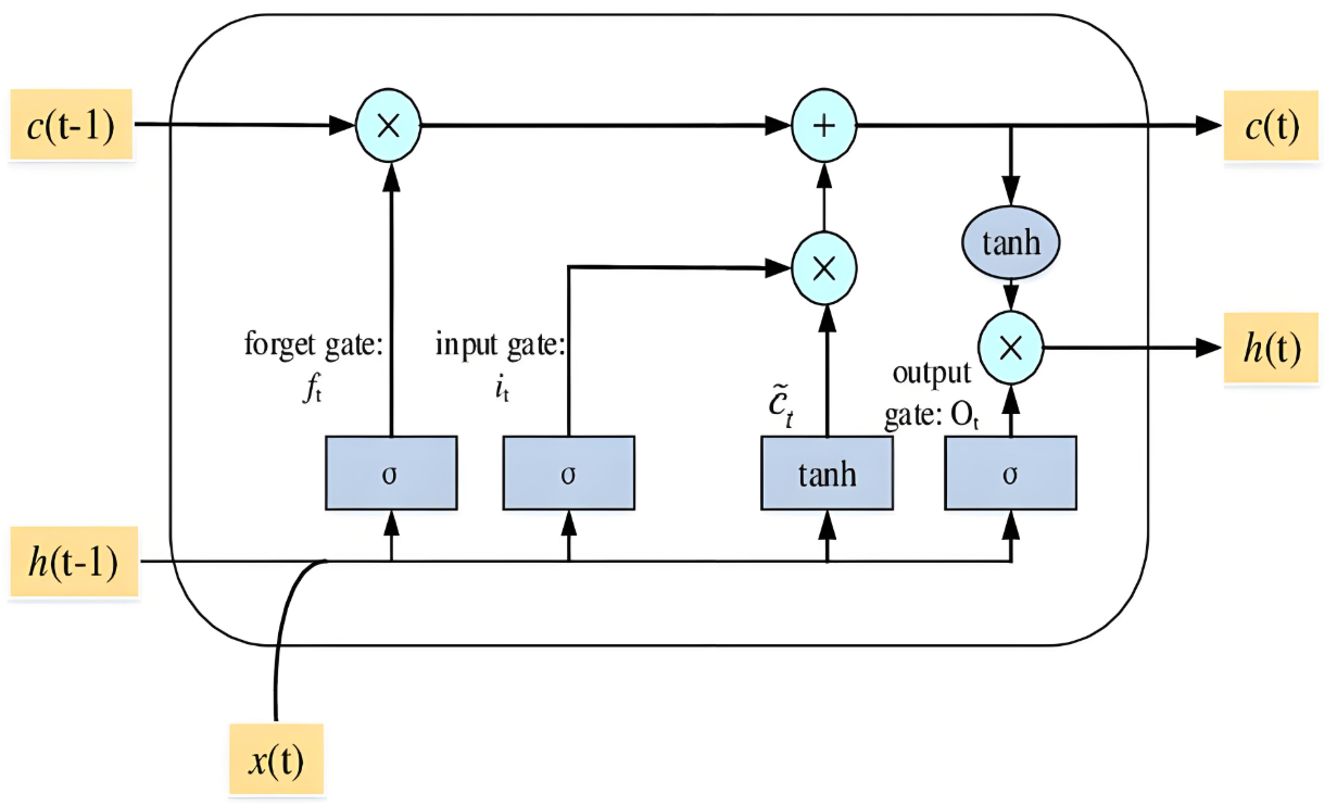
plt.title('LSTM单元结构')
plt.show()LSTM核心组件:
遗忘门:控制前一刻记忆保留程度 $f_t = \sigma(W_f \cdot [h_{t-1}, x_t] + b_f)$
输入门:控制新记忆写入程度 $i_t = \sigma(W_i \cdot [h_{t-1}, x_t] + b_i)$
候选记忆:生成新记忆内容 $\tilde{C}t = \tanh(W_C \cdot [h{t-1}, x_t] + b_C)$
细胞状态更新:$C_t = f_t \odot C_{t-1} + i_t \odot \tilde{C}_t$
输出门:控制输出内容 $o_t = \sigma(W_o \cdot [h_{t-1}, x_t] + b_o)$
隐藏状态输出:$h_t = o_t \odot \tanh(C_t)$
# 时间序列预测:正弦波
time_steps = np.linspace(0, 50, 500)
data = np.sin(time_steps)
# 创建序列数据集
def create_dataset(seq, lookback=10):
    X, y = [], []
    for i in range(len(seq)-lookback):
        X.append(seq[i:i+lookback])
        y.append(seq[i+lookback])
    return np.array(X), np.array(y)
lookback = 20
X, y = create_dataset(data, lookback)
X = X.reshape(-1, lookback, 1)  # (样本数, 时间步, 特征数)
y = y.reshape(-1, 1)
# 转换为PyTorch张量
X_tensor = torch.tensor(X, dtype=torch.float32)
y_tensor = torch.tensor(y, dtype=torch.float32)
# 定义LSTM模型
class LSTMModel(nn.Module):
    def __init__(self, input_size=1, hidden_size=64, output_size=1):
        super().__init__()
        self.lstm = nn.LSTM(input_size, hidden_size, batch_first=True)
        self.linear = nn.Linear(hidden_size, output_size)

    def forward(self, x):
        # LSTM层
        out, (h_n, c_n) = self.lstm(x)  # out: (batch, seq, hidden)

        # 只取最后一个时间步
        out = self.linear(out[:, -1, :])
        return out
# 训练配置
model = LSTMModel()
criterion = nn.MSELoss()
optimizer = torch.optim.Adam(model.parameters(), lr=0.01)
# 训练循环
epochs = 100
losses = []
for epoch in range(epochs):
    optimizer.zero_grad()
    outputs = model(X_tensor)
    loss = criterion(outputs, y_tensor)
    loss.backward()
    optimizer.step()
    losses.append(loss.item())

    if (epoch+1) % 10 == 0:
        print(f'Epoch [{epoch+1}/{epochs}], Loss: {loss.item():.6f}')
# 可视化训练损失
plt.plot(losses)
plt.title('LSTM训练损失')
plt.xlabel('Epoch')
plt.ylabel('MSE Loss')
plt.grid(True)
plt.show()
# 预测结果可视化
with torch.no_grad():
    predictions = model(X_tensor).numpy()
plt.figure(figsize=(12, 6))
plt.plot(time_steps[lookback:], data[lookback:], label='真实值')
plt.plot(time_steps[lookback:], predictions, label='预测值', alpha=0.7)
plt.title('LSTM时间序列预测')
plt.legend()
plt.grid(True)
plt.show()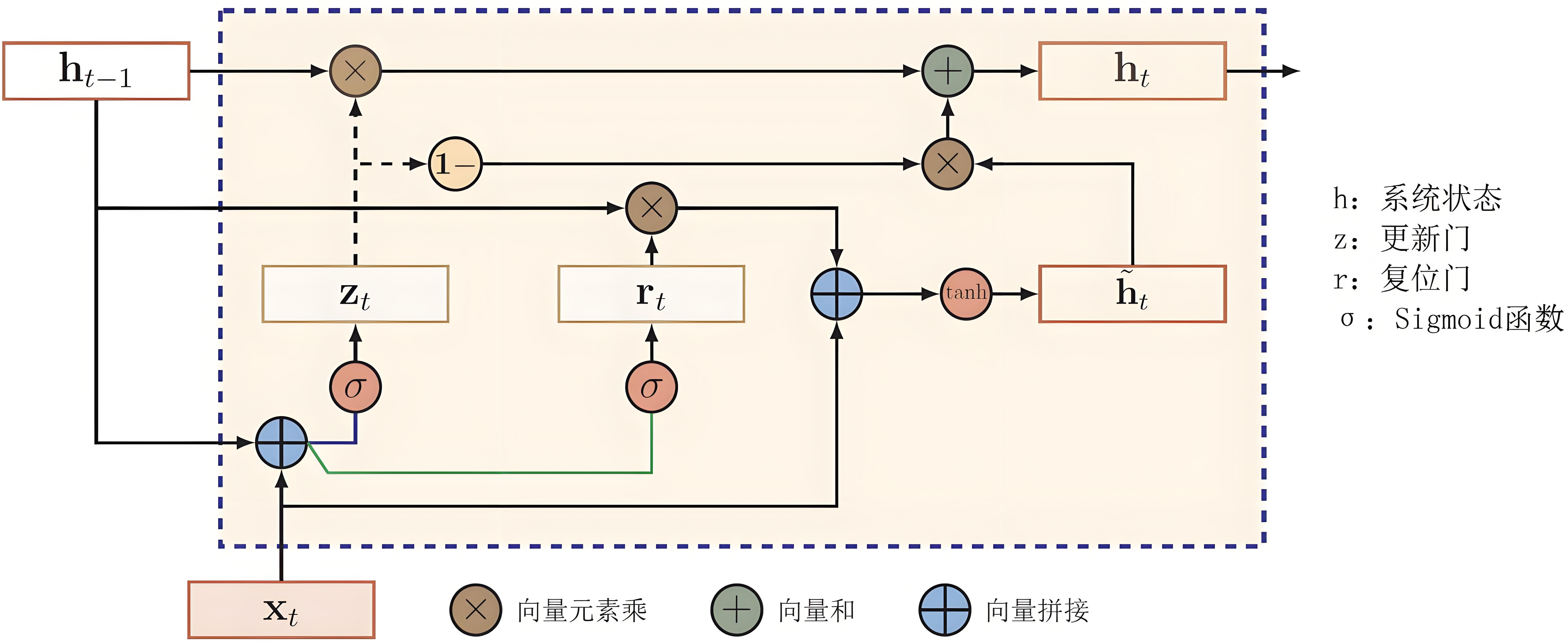
class GRUCellManual:
    def __init__(self, input_size, hidden_size):
        # 更新门参数
        self.W_xz = nn.Parameter(torch.randn(input_size, hidden_size))
        self.W_hz = nn.Parameter(torch.randn(hidden_size, hidden_size))
        self.b_z = nn.Parameter(torch.zeros(1, hidden_size))

        # 重置门参数
        self.W_xr = nn.Parameter(torch.randn(input_size, hidden_size))
        self.W_hr = nn.Parameter(torch.randn(hidden_size, hidden_size))
        self.b_r = nn.Parameter(torch.zeros(1, hidden_size))

        # 候选激活参数
        self.W_xh = nn.Parameter(torch.randn(input_size, hidden_size))
        self.W_hh = nn.Parameter(torch.randn(hidden_size, hidden_size))
        self.b_h = nn.Parameter(torch.zeros(1, hidden_size))

        self.hidden_size = hidden_size

    def forward(self, x, h_prev):
        # 更新门
        z = torch.sigmoid(x @ self.W_xz + h_prev @ self.W_hz + self.b_z)

        # 重置门
        r = torch.sigmoid(x @ self.W_xr + h_prev @ self.W_hr + self.b_r)

        # 候选激活
        h_hat = torch.tanh(x @ self.W_xh + (r * h_prev) @ self.W_hh + self.b_h)

        # 更新隐藏状态
        h_next = (1 - z) * h_prev + z * h_hat

        return h_next
# GRU结构可视化
plt.figure(figsize=(8, 6))
plt.imshow(plt.imread('gru_cell.png'))  # 实际使用时替换为GRU结构图
plt.axis('off')
plt.title('GRU单元结构')
plt.show()
GRU核心组件:
更新门:控制状态更新程度 $z_t = \sigma(W_z \cdot [h_{t-1}, x_t])$
重置门:控制历史信息重置程度 $r_t = \sigma(W_r \cdot [h_{t-1}, x_t])$
候选激活:$\tilde{h}t = \tanh(W \cdot [r_t \odot h{t-1}, x_t])$
状态更新:$h_t = (1 - z_t) \odot h_{t-1} + z_t \odot \tilde{h}_t$
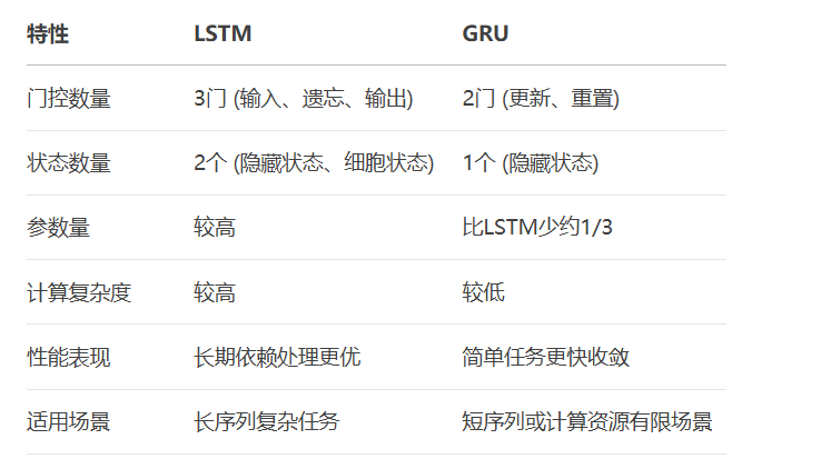
LSTM vs GRU对比:
# 文本数据预处理
text = "循环神经网络是处理序列数据的强大模型。"
chars = sorted(set(text))
char_to_idx = {ch: i for i, ch in enumerate(chars)}
idx_to_char = {i: ch for i, ch in enumerate(chars)}
# 创建训练数据
seq_length = 10
sequences = []
next_chars = []
for i in range(0, len(text) - seq_length):
    seq = text[i:i + seq_length]
    next_char = text[i + seq_length]
    sequences.append([char_to_idx[ch] for ch in seq])
    next_chars.append(char_to_idx[next_char])
# 转换为张量
X = torch.tensor(sequences, dtype=torch.long)
y = torch.tensor(next_chars, dtype=torch.long)
# 定义GRU模型
class GRUTextGenerator(nn.Module):
    def __init__(self, vocab_size, embedding_dim, hidden_size):
        super().__init__()
        self.embedding = nn.Embedding(vocab_size, embedding_dim)
        self.gru = nn.GRU(embedding_dim, hidden_size, batch_first=True)
        self.fc = nn.Linear(hidden_size, vocab_size)

    def forward(self, x, h=None):
        # 嵌入层
        x = self.embedding(x)

        # GRU层
        if h is None:
            out, h = self.gru(x)
        else:
            out, h = self.gru(x, h)

        # 全连接层
        out = self.fc(out[:, -1, :])  # 取最后一个时间步
        return out, h

    def generate(self, start_str, length=100, temperature=0.8):
        # 初始化隐藏状态
        h = None
        input_seq = [char_to_idx[ch] for ch in start_str]
        generated_chars = list(start_str)

        # 生成文本
        for _ in range(length):
            x = torch.tensor([input_seq[-seq_length:]], dtype=torch.long)
            logits, h = self.forward(x, h)

            # 应用温度参数
            logits = logits / temperature
            probs = nn.functional.softmax(logits, dim=-1)

            # 采样下一个字符
            next_idx = torch.multinomial(probs, 1).item()
            next_char = idx_to_char[next_idx]

            generated_chars.append(next_char)
            input_seq.append(next_idx)

        return ''.join(generated_chars)
# 训练配置
vocab_size = len(chars)
embedding_dim = 32
hidden_size = 128
model = GRUTextGenerator(vocab_size, embedding_dim, hidden_size)
criterion = nn.CrossEntropyLoss()
optimizer = torch.optim.Adam(model.parameters(), lr=0.005)
# 训练循环
epochs = 500
for epoch in range(epochs):
    optimizer.zero_grad()
    output, _ = model(X)
    loss = criterion(output, y)
    loss.backward()
    optimizer.step()

    if (epoch+1) % 50 == 0:
        print(f'Epoch [{epoch+1}/{epochs}], Loss: {loss.item():.4f}')

        # 示例文本生成
        generated = model.generate("循环神经", length=20)
        print(f"生成文本: {generated}")
# 最终文本生成
print("\n最终生成结果:")
print(model.generate("神经网络", length=100, temperature=0.7))
bidirectional_rnn = nn.RNN(input_size=10, hidden_size=16,
                          bidirectional=True, batch_first=True)
同时考虑过去和未来信息
适用于需要上下文理解的任务
深度RNN:
deep_rnn = nn.RNN(input_size=10, hidden_size=16,
                 num_layers=3, batch_first=True)
Attention机制:
class AttentionRNN(nn.Module):
    def __init__(self, input_size, hidden_size):
        super().__init__()
        self.rnn = nn.GRU(input_size, hidden_size, batch_first=True)
        self.attention = nn.Linear(hidden_size * 2, 1)
        self.fc = nn.Linear(hidden_size, 1)

    def forward(self, x):
        outputs, _ = self.rnn(x)  # (batch, seq, hidden)

        # 注意力机制
        seq_len = outputs.size(1)
        hidden_repeat = outputs[:, -1:, :].repeat(1, seq_len, 1)
        attention_input = torch.cat((outputs, hidden_repeat), dim=2)
        attention_scores = torch.softmax(self.attention(attention_input), dim=1)
        context = torch.sum(attention_scores * outputs, dim=1)

        return self.fc(context)
动态关注重要时间步
提升长序列处理能力
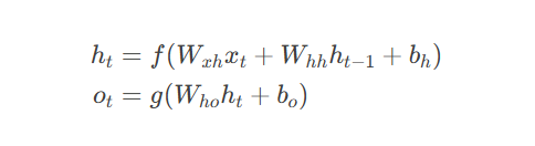
RNN核心公式:
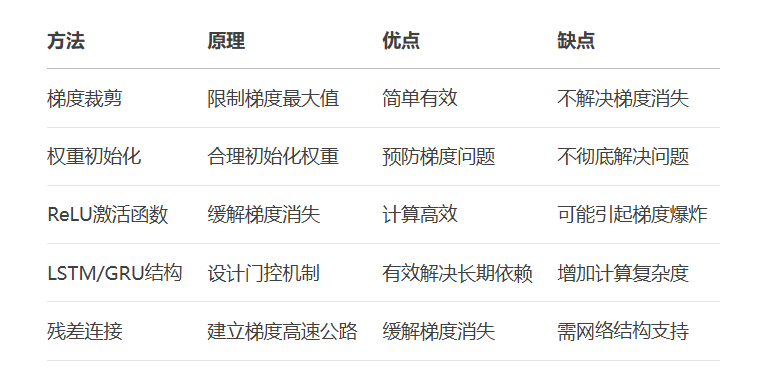
梯度问题解决方案:
graph LR
A[梯度消失/爆炸] --> B[梯度裁剪]
A --> C[权重初始化]
A --> D[ReLU激活]
A --> E[LSTM/GRU]
A --> F[残差连接]
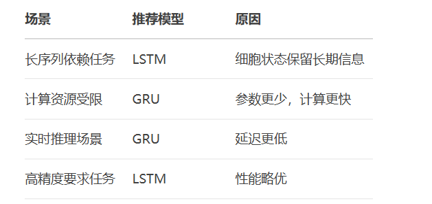
LSTM/GRU选择指南:
RNN训练最佳实践:
使用梯度裁剪防止爆炸:nn.utils.clip_grad_norm_(model.parameters(), max_norm=1.0)
选择合适的序列长度(不宜过长)
使用双向RNN获取上下文信息
结合注意力机制提升性能
使用学习率调度器优化训练
通过掌握RNN、LSTM和GRU的原理与实践,你已具备处理序列数据的基础能力。下一步可探索Transformer架构、注意力机制等更先进的序列建模技术!更多AI大模型应用开发学习视频内容及资料,尽在聚客AI学院。