本文系统讲解神经网络核心原理,涵盖感知机模型、激活函数、损失函数和反向传播算法,结合数学推导、可视化图解和代码实现,帮你彻底掌握神经网络工作机制。
import numpy as np
import matplotlib.pyplot as plt
class Perceptron:
    def __init__(self, input_size, lr=0.01):
        self.weights = np.random.randn(input_size)
        self.bias = np.random.randn()
        self.lr = lr

    def activate(self, x):
        # 阶跃函数
        return 1 if x >= 0 else 0

    def forward(self, inputs):
        summation = np.dot(inputs, self.weights) + self.bias
        return self.activate(summation)

    def train(self, inputs, target):
        prediction = self.forward(inputs)
        error = target - prediction

        # 权重更新
        self.weights += self.lr * error * inputs
        self.bias += self.lr * error

        return error
# 创建AND逻辑数据集
X = np.array([[0,0], [0,1], [1,0], [1,1]])
y = np.array([0, 0, 0, 1])
# 训练感知机
perceptron = Perceptron(input_size=2, lr=0.1)
epochs = 10
for epoch in range(epochs):
    errors = 0
    for i in range(len(X)):
        error = perceptron.train(X[i], y[i])
        errors += abs(error)

    print(f"Epoch {epoch+1}, Total Error: {errors}")
    if errors == 0:
        break
# 测试感知机
print("\n测试结果:")
for i in range(len(X)):
    pred = perceptron.forward(X[i])
print(f"输入: {X[i]}, 预测: {pred}, 期望: {y[i]}")# 可视化决策边界
x_min, x_max = -0.5, 1.5
y_min, y_max = -0.5, 1.5
xx, yy = np.meshgrid(np.arange(x_min, x_max, 0.01),
np.arange(y_min, y_max, 0.01))
Z = np.array([perceptron.forward(np.array([x, y]))
for x, y in zip(xx.ravel(), yy.ravel())])
Z = Z.reshape(xx.shape)
plt.figure(figsize=(8,6))
plt.contourf(xx, yy, Z, alpha=0.4)
plt.scatter(X[:,0], X[:,1], c=y, s=100, edgecolors='k')
plt.title("感知机决策边界")
plt.xlabel("输入1")
plt.ylabel("输入2")
plt.grid(True)
plt.show()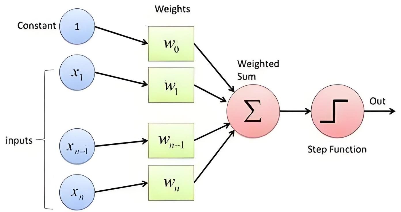
数学原理:
输出 = f(w·x + b)
其中:
w = 权重向量
x = 输入向量
b = 偏置项
f = 激活函数(阶跃函数)
import torch
import torch.nn.functional as F
# 定义常用激活函数
def sigmoid(x):
    return 1 / (1 + np.exp(-x))
def relu(x):
    return np.maximum(0, x)
def tanh(x):
    return np.tanh(x)
def softmax(x):
    exp_x = np.exp(x - np.max(x))
    return exp_x / exp_x.sum(axis=0)
# 可视化
x = np.linspace(-5, 5, 100)
plt.figure(figsize=(12, 8))
plt.subplot(2, 2, 1)
plt.plot(x, sigmoid(x))
plt.title("Sigmoid"), plt.grid(True)
plt.subplot(2, 2, 2)
plt.plot(x, relu(x))
plt.title("ReLU"), plt.grid(True)
plt.subplot(2, 2, 3)
plt.plot(x, tanh(x))
plt.title("Tanh"), plt.grid(True)
plt.subplot(2, 2, 4)
plt.plot(x, softmax(x))
plt.title("Softmax"), plt.grid(True)
plt.tight_layout()
plt.show()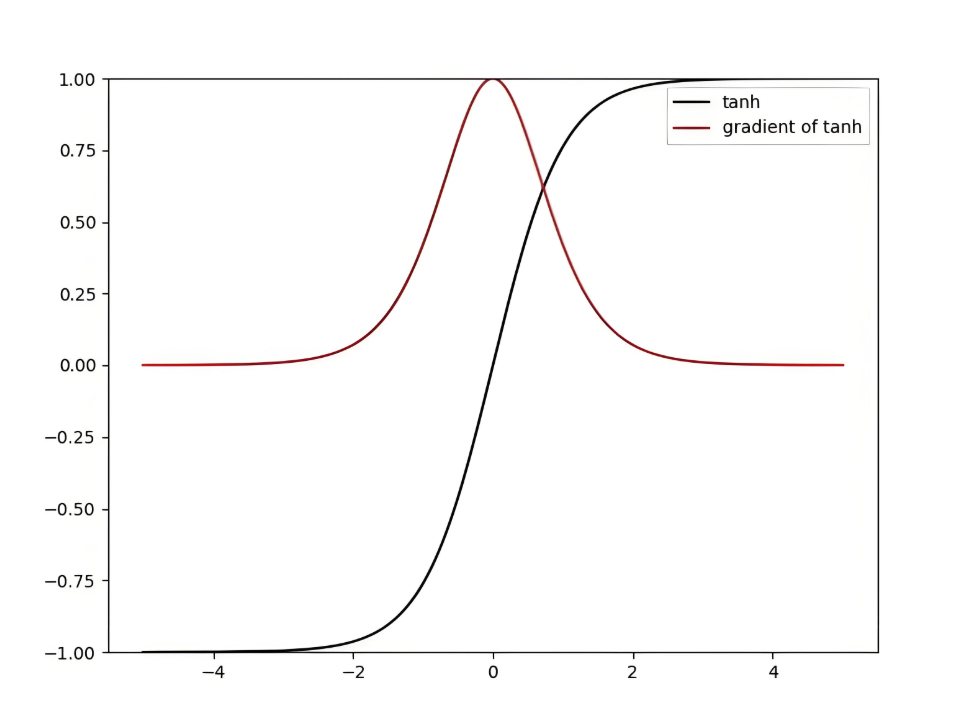
# 激活函数导数
def sigmoid_derivative(x):
    s = sigmoid(x)
    return s * (1 - s)
def relu_derivative(x):
    return np.where(x > 0, 1, 0)
def tanh_derivative(x):
    return 1 - np.tanh(x)**2
# 可视化导数
x = np.linspace(-3, 3, 100)
plt.figure(figsize=(12, 4))
plt.subplot(1, 3, 1)
plt.plot(x, sigmoid_derivative(x))
plt.title("Sigmoid导数")
plt.subplot(1, 3, 2)
plt.plot(x, relu_derivative(x))
plt.title("ReLU导数")
plt.subplot(1, 3, 3)
plt.plot(x, tanh_derivative(x))
plt.title("Tanh导数")
plt.tight_layout()
plt.show()# 均方误差 (MSE)
def mse_loss(y_true, y_pred):
return np.mean((y_true - y_pred)**2)
# 交叉熵损失
def cross_entropy_loss(y_true, y_pred, epsilon=1e-12):
y_pred = np.clip(y_pred, epsilon, 1. - epsilon)
return -np.mean(y_true * np.log(y_pred) + (1 - y_true) * np.log(1 - y_pred))
# 分类交叉熵
def categorical_crossentropy(y_true, y_pred, epsilon=1e-12):
y_pred = np.clip(y_pred, epsilon, 1. - epsilon)
return -np.sum(y_true * np.log(y_pred)) / y_true.shape[0]
# 可视化损失函数
y_true = np.array([1, 0, 1])
y_pred = np.linspace(0, 1, 100)
# MSE可视化
plt.figure(figsize=(12, 4))
plt.subplot(1, 3, 1)
plt.plot(y_pred, mse_loss(np.array([1]*100), y_pred))
plt.title("MSE (y_true=1)")
plt.xlabel("预测值"), plt.ylabel("损失")
# 二分类交叉熵
plt.subplot(1, 3, 2)
plt.plot(y_pred, cross_entropy_loss(np.array([1]*100), y_pred))
plt.title("二分类交叉熵 (y_true=1)")
# 多分类交叉熵
plt.subplot(1, 3, 3)
y_true_multi = np.eye(3) # 3个类别的one-hot编码
y_pred_multi = np.array([np.linspace(0.01, 0.99, 100)]*3).T
losses = [categorical_crossentropy(y_true_multi, np.array([p, (1-p)/2, (1-p)/2])) for p in y_pred]
plt.plot(y_pred, losses)
plt.title("多分类交叉熵 (真实类别0)")
plt.tight_layout()
plt.show()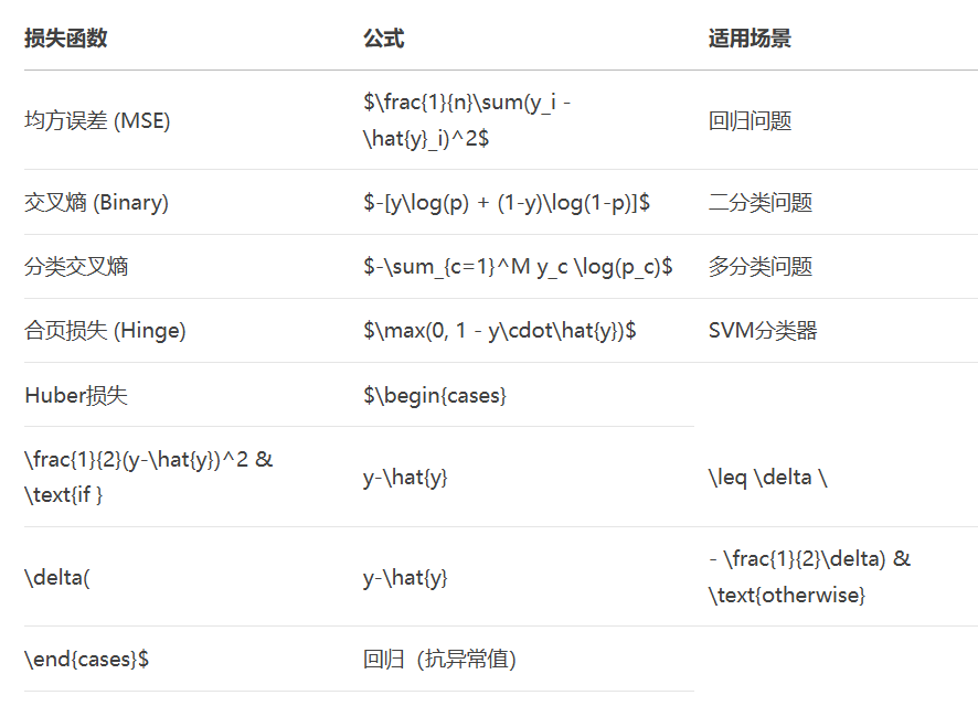
考虑一个简单网络:
输入层 (x) → 隐藏层 (h = σ(W1·x + b1)) → 输出层 (y = W2·h + b2)
损失函数 L = 1/2(y - t)^2
反向传播公式推导:
输出层梯度:
$\frac{\partial L}{\partial y} = y - t$
$\frac{\partial L}{\partial W2} = \frac{\partial L}{\partial y} \cdot h^T$
$\frac{\partial L}{\partial b2} = \frac{\partial L}{\partial y}$
隐藏层梯度:
$\frac{\partial L}{\partial h} = W2^T \cdot \frac{\partial L}{\partial y}$
$\frac{\partial L}{\partial z} = \frac{\partial L}{\partial h} \odot \sigma'(z)$
$\frac{\partial L}{\partial W1} = \frac{\partial L}{\partial z} \cdot x^T$
$\frac{\partial L}{\partial b1} = \frac{\partial L}{\partial z}$
# 神经网络参数
W1 = np.random.randn(2, 3)  # 输入层到隐藏层
b1 = np.random.randn(3)
W2 = np.random.randn(3, 1)  # 隐藏层到输出层
b2 = np.random.randn(1)
learning_rate = 0.1
# 前向传播函数
def forward(x):
    z1 = np.dot(x, W1) + b1
    h = np.tanh(z1)  # 隐藏层激活
    z2 = np.dot(h, W2) + b2
    return z2, h  # 返回输出和隐藏层状态
# 反向传播函数
def backward(x, y_true, y_pred, h):
    # 计算损失梯度
    dL_dy = y_pred - y_true

    # 输出层梯度
    dL_dW2 = np.dot(h.T, dL_dy)
    dL_db2 = np.sum(dL_dy, axis=0)

    # 隐藏层梯度
    dL_dh = np.dot(dL_dy, W2.T)
    dL_dz1 = dL_dh * (1 - np.tanh(h)**2)  # tanh导数

    # 输入层梯度
    dL_dW1 = np.dot(x.T, dL_dz1)
    dL_db1 = np.sum(dL_dz1, axis=0)

    return dL_dW1, dL_db1, dL_dW2, dL_db2
# 训练数据
X = np.array([[0,0], [0,1], [1,0], [1,1]])
y = np.array([[0], [1], [1], [0]])  # XOR问题
# 训练循环
for epoch in range(10000):
    total_loss = 0
    for i in range(len(X)):
        # 前向传播
        x_in = X[i].reshape(1, -1)
        y_true = y[i].reshape(1, -1)

        y_pred, h = forward(x_in)
        loss = 0.5 * (y_pred - y_true)**2
        total_loss += loss.item()

        # 反向传播
        dW1, db1, dW2, db2 = backward(x_in, y_true, y_pred, h)

        # 更新参数
        W1 -= learning_rate * dW1
        b1 -= learning_rate * db1
        W2 -= learning_rate * dW2
        b2 -= learning_rate * db2

    if epoch % 1000 == 0:
        print(f"Epoch {epoch}, Loss: {total_loss/len(X)}")
# 测试
print("\nXOR问题测试:")
for i in range(len(X)):
    y_pred, _ = forward(X[i].reshape(1, -1))
print(f"输入: {X[i]}, 预测: {y_pred.item():.4f}, 期望: {y[i][0]}")graph LR A[输入 x] --> B[加权和 z1 = W1·x + b1] B --> C[激活 h = tanh z1] C --> D[加权和 z2 = W2·h + b2] D --> E[输出 y] E --> F[损失 L = 1/2 y-t 2] F -- dL/dy --> D D -- dL/dW2 = dL/dy·hT --> W2 D -- dL/db2 = dL/dy --> b2 D -- dL/dh = W2T·dL/dy --> C C -- dL/dz1 = dL/dh * tanh' --> B B -- dL/dW1 = dL/dz1·xT --> W1 B -- dL/db1 = dL/dz1 --> b1
import torch
import torch.nn as nn
import torch.optim as optim
from torchvision import datasets, transforms
from torch.utils.data import DataLoader
# 定义神经网络
class NeuralNet(nn.Module):
    def __init__(self, input_size, hidden_size, output_size):
        super().__init__()
        self.fc1 = nn.Linear(input_size, hidden_size)
        self.relu = nn.ReLU()
        self.fc2 = nn.Linear(hidden_size, output_size)

    def forward(self, x):
        x = x.view(x.size(0), -1)  # 展平
        x = self.fc1(x)
        x = self.relu(x)
        x = self.fc2(x)
        return x
# 加载MNIST数据集
transform = transforms.Compose([
    transforms.ToTensor(),
    transforms.Normalize((0.1307,), (0.3081,))
])
train_data = datasets.MNIST('./data', train=True, download=True, transform=transform)
test_data = datasets.MNIST('./data', train=False, transform=transform)
train_loader = DataLoader(train_data, batch_size=64, shuffle=True)
test_loader = DataLoader(test_data, batch_size=1000)
# 初始化模型
device = torch.device("cuda" if torch.cuda.is_available() else "cpu")
model = NeuralNet(28*28, 256, 10).to(device)
criterion = nn.CrossEntropyLoss()
optimizer = optim.Adam(model.parameters(), lr=0.001)
# 训练函数
def train(epoch):
    model.train()
    for batch_idx, (data, target) in enumerate(train_loader):
        data, target = data.to(device), target.to(device)

        # 前向传播
        output = model(data)
        loss = criterion(output, target)

        # 反向传播
        optimizer.zero_grad()
        loss.backward()
        optimizer.step()

        if batch_idx % 100 == 0:
            print(f'Train Epoch: {epoch} [{batch_idx*len(data)}/{len(train_loader.dataset)}'
                  f' ({100.*batch_idx/len(train_loader):.0f}%)]\tLoss: {loss.item():.6f}')
# 测试函数
def test():
    model.eval()
    test_loss = 0
    correct = 0
    with torch.no_grad():
        for data, target in test_loader:
            data, target = data.to(device), target.to(device)
            output = model(data)
            test_loss += criterion(output, target).item()
            pred = output.argmax(dim=1, keepdim=True)
            correct += pred.eq(target.view_as(pred)).sum().item()

    test_loss /= len(test_loader.dataset)
    accuracy = 100. * correct / len(test_loader.dataset)
    print(f'\n测试集: 平均损失: {test_loss:.4f}, 准确率: {correct}/{len(test_loader.dataset)} ({accuracy:.2f}%)\n')
    return accuracy
# 训练循环
accuracies = []
for epoch in range(1, 11):
    train(epoch)
    acc = test()
    accuracies.append(acc)
# 可视化训练过程
plt.plot(accuracies)
plt.title('MNIST分类准确率')
plt.xlabel('Epochs')
plt.ylabel('Accuracy (%)')
plt.grid(True)
plt.show()graph TD
A[输入数据] --> B[前向传播]
B --> C[计算损失]
C --> D[反向传播]
D --> E[参数更新]
E --> F{达到停止条件?}
F -- 是 --> G[模型部署]
F -- 否 --> B输出 = f(∑(w_i * x_i) + b)
其中f为激活函数,w为权重,b为偏置
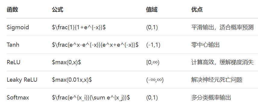
激活函数选择指南:
隐藏层:优先使用ReLU及其变体(计算高效)
二分类输出层:Sigmoid函数
多分类输出层:Softmax函数
回归输出层:线性激活(无激活函数)
损失函数选择原则:
回归问题:MSE(均方误差)
二分类问题:二元交叉熵
多分类问题:分类交叉熵
异常值处理:Huber损失
反向传播四步骤:
# 1. 前向传播计算预测值
outputs = model(inputs)
# 2. 计算损失
loss = criterion(outputs, targets)
# 3. 反向传播计算梯度
optimizer.zero_grad()  # 清空历史梯度
loss.backward()        # 自动计算梯度
# 4. 更新参数
optimizer.step()       # 根据梯度更新权重
神经网络设计原则:
输入层节点数 = 特征维度
输出层节点数 = 类别数(分类)或1(回归)
隐藏层节点数:64-1024(根据问题复杂度调整)
隐藏层数量:1-3层(简单问题),>10层(深度学习)
通过掌握这些神经网络基础,你已经为学习卷积神经网络、循环神经网络等高级模型奠定了坚实基础!更多AI大模型应用开发学习视频内容和资料,尽在聚客AI学院。