掌握监督/无监督学习、过拟合/欠拟合、偏差/方差、评估指标和交叉验证是机器学习入门的核心基础。本文通过理论解析+可视化+代码实战,帮你构建系统认知框架。
import matplotlib.pyplot as plt
import numpy as np
from sklearn.datasets import make_classification, make_blobs
# 生成数据
X_sup, y_sup = make_classification(n_samples=100, n_features=2, n_classes=3,
                                  n_redundant=0, n_clusters_per_class=1)
X_unsup, _ = make_blobs(n_samples=100, centers=3, random_state=42)
# 可视化
fig, (ax1, ax2) = plt.subplots(1, 2, figsize=(15, 6))
# 监督学习(带标签)
ax1.scatter(X_sup[:, 0], X_sup[:, 1], c=y_sup, cmap='viridis', edgecolors='k')
ax1.set_title('监督学习:带标签数据', fontsize=14)
ax1.set_xlabel('特征1'), ax1.set_ylabel('特征2')
# 无监督学习(无标签)
ax2.scatter(X_unsup[:, 0], X_unsup[:, 1], c='blue', edgecolors='k')
ax2.set_title('无监督学习:未标记数据', fontsize=14)
ax2.set_xlabel('特征1'), ax2.set_ylabel('特征2')
plt.tight_layout()
plt.show()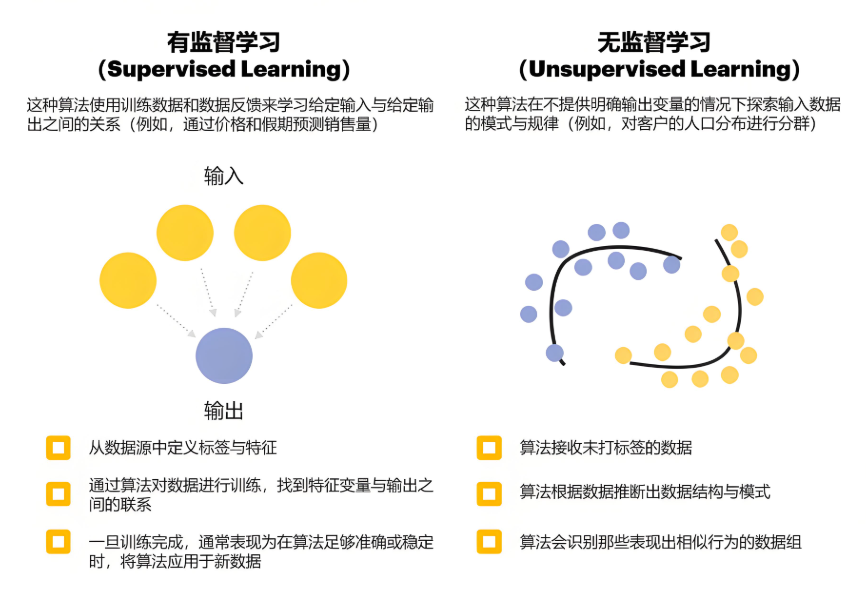
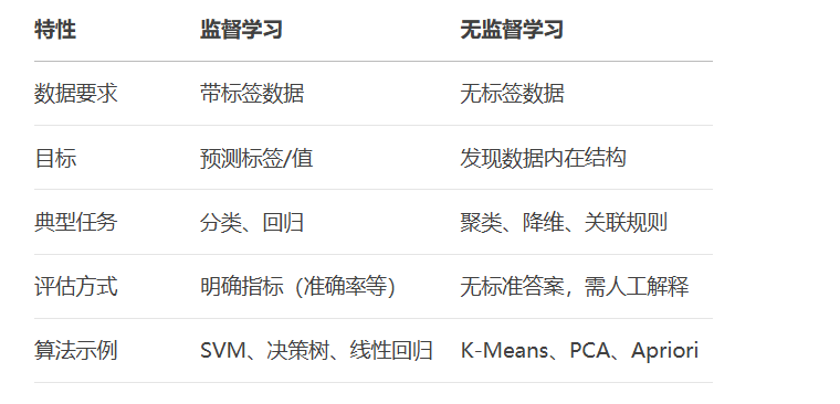
关键区别:
from sklearn.pipeline import make_pipeline
from sklearn.preprocessing import PolynomialFeatures
from sklearn.linear_model import LinearRegression
# 生成非线性数据
np.random.seed(42)
X = np.linspace(0, 10, 100)
y = np.sin(X) + 0.3 * np.random.randn(100)
# 不同复杂度模型
degrees = [1, 4, 15]
models = {}
plt.figure(figsize=(15, 5))
for i, degree in enumerate(degrees):
    ax = plt.subplot(1, 3, i+1)

    # 多项式回归
    model = make_pipeline(PolynomialFeatures(degree), LinearRegression())
    model.fit(X[:, np.newaxis], y)
    models[degree] = model

    # 预测
    X_test = np.linspace(0, 10, 1000)
    y_test = model.predict(X_test[:, np.newaxis])

    # 可视化
    ax.scatter(X, y, alpha=0.5, label='真实数据')
    ax.plot(X_test, y_test, 'r-', linewidth=2, label='模型预测')
    ax.set_title(f'多项式阶数: {degree}')
    ax.set_ylim(-2, 2)
    ax.legend()
plt.tight_layout()
plt.show()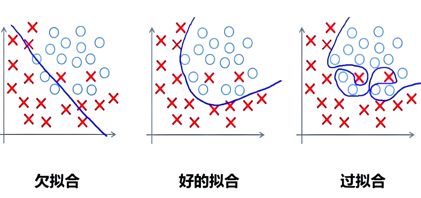
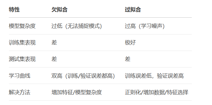
核心特征对比:
总误差可分解为:
总误差=偏差2+方差+不可约误差
偏差:模型预测与真实值的系统性偏离
方差:模型对训练数据变化的敏感度
不可约误差:数据本身的噪声
from mlxtend.evaluate import bias_variance_decomp
from sklearn.tree import DecisionTreeRegressor
from sklearn.ensemble import BaggingRegressor
# 生成数据
X = np.random.rand(100, 1) * 10
y = np.sin(X).ravel() + np.random.normal(0, 0.2, 100)
# 不同模型对比
models = {
    "高偏差(线性回归)": LinearRegression(),
    "高方差(决策树)": DecisionTreeRegressor(max_depth=10),
    "平衡(随机森林)": BaggingRegressor(n_estimators=50)
}
plt.figure(figsize=(15, 10))
for i, (name, model) in enumerate(models.items()):
    # 计算偏差方差
    avg_expected_loss, avg_bias, avg_var = bias_variance_decomp(
        model, X, y, X, y, num_rounds=10)

    # 可视化
    ax = plt.subplot(2, 2, i+1)
    model.fit(X, y)
    y_pred = model.predict(X)

    ax.scatter(X, y, alpha=0.7, label='真实数据')
    ax.plot(np.sort(X, axis=0), y_pred[np.argsort(X, axis=0).ravel()],
            'r-', linewidth=2, label='模型预测')
    ax.set_title(f"{name}\n偏差={avg_bias:.3f}, 方差={avg_var:.3f}")
    ax.legend()
plt.tight_layout()
plt.show()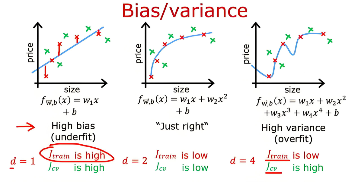
权衡策略:
高偏差:增加模型复杂度、添加特征、减少正则化
高方差:增加训练数据、简化模型、增强正则化、使用集成方法
from sklearn.metrics import confusion_matrix, precision_recall_curve, roc_curve, auc
from sklearn.datasets import make_classification
from sklearn.model_selection import train_test_split
from sklearn.linear_model import LogisticRegression
# 生成分类数据
X, y = make_classification(n_samples=1000, n_classes=2, weights=[0.9, 0.1], random_state=42)
X_train, X_test, y_train, y_test = train_test_split(X, y, test_size=0.3)
# 训练模型
model = LogisticRegression()
model.fit(X_train, y_train)
y_pred = model.predict(X_test)
y_proba = model.predict_proba(X_test)[:, 1]
# 混淆矩阵
cm = confusion_matrix(y_test, y_pred)
tn, fp, fn, tp = cm.ravel()
# 指标计算
accuracy = (tp + tn) / (tp + tn + fp + fn)
precision = tp / (tp + fp)
recall = tp / (tp + fn)
f1 = 2 * (precision * recall) / (precision + recall)
print(f"准确率: {accuracy:.3f}")
print(f"精确率: {precision:.3f}")
print(f"召回率: {recall:.3f}")
print(f"F1分数: {f1:.3f}")
# ROC曲线
fpr, tpr, _ = roc_curve(y_test, y_proba)
roc_auc = auc(fpr, tpr)
# PR曲线
precision_curve, recall_curve, _ = precision_recall_curve(y_test, y_proba)
# 可视化
fig, (ax1, ax2) = plt.subplots(1, 2, figsize=(15, 6))
# ROC曲线
ax1.plot(fpr, tpr, color='darkorange', lw=2, label=f'ROC曲线 (AUC = {roc_auc:.2f})')
ax1.plot([0, 1], [0, 1], color='navy', lw=2, linestyle='--')
ax1.set_xlim([0.0, 1.0]), ax1.set_ylim([0.0, 1.05])
ax1.set_xlabel('假正例率 (FPR)'), ax1.set_ylabel('真正例率 (TPR)')
ax1.set_title('ROC曲线'), ax1.legend()
# PR曲线
ax2.plot(recall_curve, precision_curve, color='blue', lw=2)
ax2.set_xlim([0.0, 1.0]), ax2.set_ylim([0.0, 1.05])
ax2.set_xlabel('召回率'), ax2.set_ylabel('精确率')
ax2.set_title('精确率-召回率曲线')
plt.tight_layout()
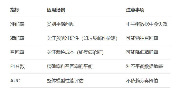
plt.show()指标使用场景:
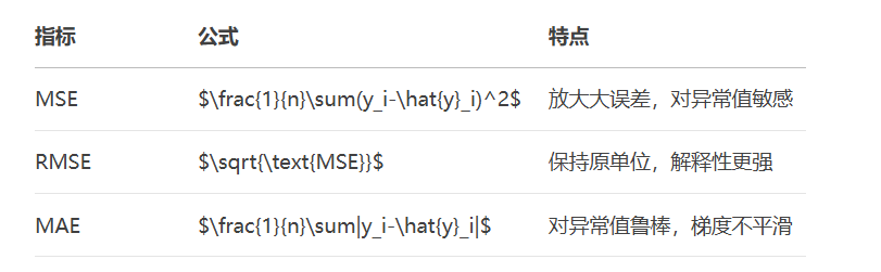
4.2 回归指标:MSE vs MAE
from sklearn.metrics import mean_squared_error, mean_absolute_error
# 生成回归数据
X = np.random.rand(100, 1) * 10
y = 2.5 * X + 1 + np.random.randn(100, 1) * 2
# 添加异常值
y[10] = 50
y[20] = 60
# 计算指标
y_pred = 2.7 * X + 0.8  # 模拟预测值
mse = mean_squared_error(y, y_pred)
mae = mean_absolute_error(y, y_pred)
print(f"MSE: {mse:.2f}")
print(f"RMSE: {np.sqrt(mse):.2f}")
print(f"MAE: {mae:.2f}")
# 可视化对比
plt.figure(figsize=(10, 6))
plt.scatter(X, y, alpha=0.7, label='真实值')
plt.plot(X, y_pred, 'r-', linewidth=2, label='预测值')
# 标注异常值
plt.annotate('异常值影响MSE', xy=(X[10], y[10]), xytext=(3, 40),
             arrowprops=dict(facecolor='black', shrink=0.05))
plt.title('回归指标对比 (MSE vs MAE)')
plt.xlabel('特征X'), plt.ylabel('目标y')
plt.legend()
plt.show()
回归指标对比:
from sklearn.model_selection import KFold, cross_val_score
from sklearn.datasets import load_iris
from sklearn.svm import SVC
# 加载数据
iris = load_iris()
X, y = iris.data, iris.target
# 创建模型
model = SVC(kernel='linear', C=1)
# 5折交叉验证
kf = KFold(n_splits=5, shuffle=True, random_state=42)
scores = cross_val_score(model, X, y, cv=kf, scoring='accuracy')
# 可视化
plt.figure(figsize=(10, 6))
plt.bar(range(1, 6), scores, color='skyblue')
plt.axhline(y=np.mean(scores), color='r', linestyle='--',
            label=f'平均准确率: {np.mean(scores):.3f}')
plt.xlabel('折数')
plt.ylabel('准确率')
plt.title('5折交叉验证结果')
plt.ylim(0.8, 1.0)
plt.legend()
plt.show()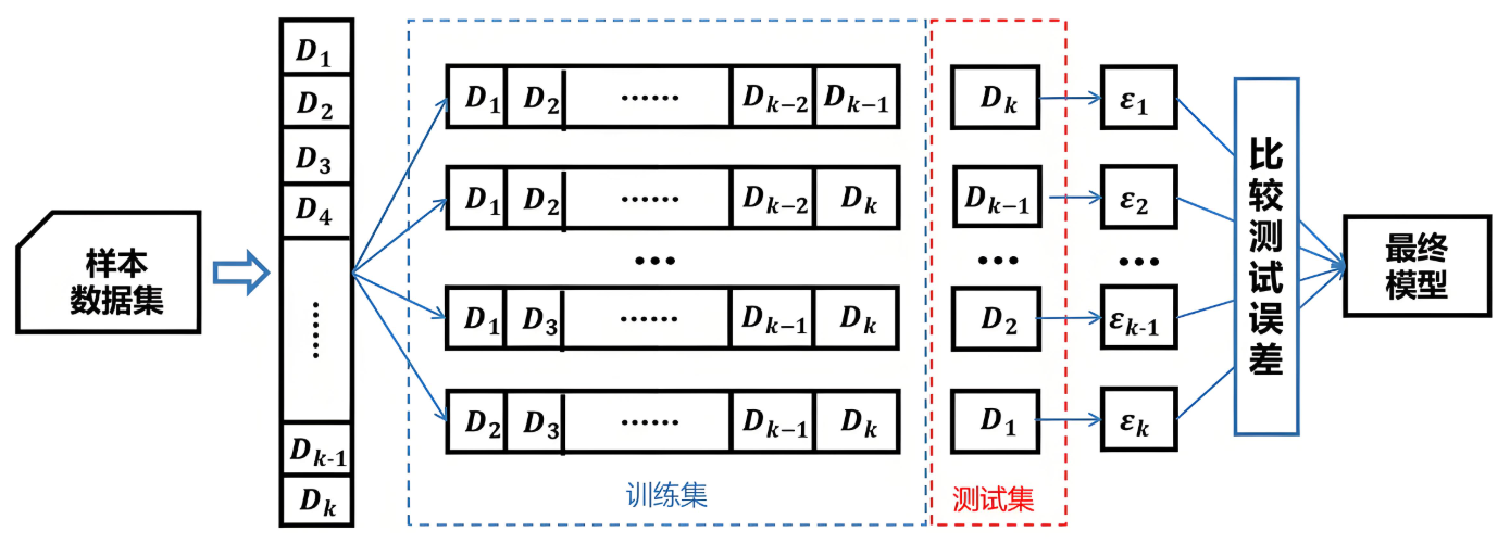
from sklearn.model_selection import StratifiedKFold, LeaveOneOut
# 分层K折(保持类别比例)
stratified_kf = StratifiedKFold(n_splits=5)
strat_scores = cross_val_score(model, X, y, cv=stratified_kf)
# 留一法交叉验证
loo = LeaveOneOut()
loo_scores = cross_val_score(model, X, y, cv=loo)
print(f"标准K折平均准确率: {np.mean(scores):.3f}")
print(f"分层K折平均准确率: {np.mean(strat_scores):.3f}")
print(f"留一法平均准确率: {np.mean(loo_scores):.3f}")
交叉验证方法对比:

from sklearn.datasets import load_breast_cancer
from sklearn.preprocessing import StandardScaler
from sklearn.model_selection import train_test_split, GridSearchCV
from sklearn.svm import SVC
from sklearn.metrics import classification_report
# 加载乳腺癌数据集
data = load_breast_cancer()
X, y = data.data, data.target
# 数据标准化
scaler = StandardScaler()
X_scaled = scaler.fit_transform(X)
# 划分训练测试集
X_train, X_test, y_train, y_test = train_test_split(X_scaled, y, test_size=0.2, random_state=42)
# 参数网格搜索
param_grid = {
    'C': [0.1, 1, 10, 100],
    'gamma': [1, 0.1, 0.01, 0.001],
    'kernel': ['rbf', 'linear']
}
# 交叉验证网格搜索
grid = GridSearchCV(SVC(), param_grid, refit=True, cv=5, scoring='f1')
grid.fit(X_train, y_train)
# 最佳模型评估
best_model = grid.best_estimator_
y_pred = best_model.predict(X_test)
print(f"最佳参数: {grid.best_params_}")
print(classification_report(y_test, y_pred))
# 学习曲线
from sklearn.model_selection import learning_curve
train_sizes, train_scores, test_scores = learning_curve(
    best_model, X_scaled, y, cv=5, scoring='accuracy',
    train_sizes=np.linspace(0.1, 1.0, 10))
# 可视化学习曲线
plt.figure(figsize=(10, 6))
plt.plot(train_sizes, np.mean(train_scores, axis=1), 'o-', label="训练准确率")
plt.plot(train_sizes, np.mean(test_scores, axis=1), 'o-', label="验证准确率")
plt.fill_between(train_sizes,
                 np.mean(train_scores, axis=1) - np.std(train_scores, axis=1),
                 np.mean(train_scores, axis=1) + np.std(train_scores, axis=1),
                 alpha=0.1)
plt.fill_between(train_sizes,
                 np.mean(test_scores, axis=1) - np.std(test_scores, axis=1),
                 np.mean(test_scores, axis=1) + np.std(test_scores, axis=1),
                 alpha=0.1)
plt.xlabel('训练样本数')
plt.ylabel('准确率')
plt.title('学习曲线')
plt.legend()
plt.grid(True)
plt.show()
建模最佳实践:
数据标准化:消除特征量纲影响
参数调优:使用网格搜索+交叉验证
模型评估:多指标综合判断(尤其不平衡数据)
学习曲线:诊断过拟合/欠拟合
特征工程:持续优化特征表示
有标签数据 → 监督学习
无标签数据 → 无监督学习
部分标签数据 → 半监督学习
模型诊断与优化:
graph LR
A[高训练误差] --> B[欠拟合]
B --> C[增加模型复杂度/特征]
A[高训练误差] --> D{验证误差}
D -->|高| B
D -->|低| E[过拟合]
E --> F[增加数据/正则化/简化模型]评估指标选择原则:
类别平衡 → 准确率
关注假阳性 → 精确率
关注假阴性 → 召回率
综合评估 → F1/AUC
异常值敏感 → MAE > MSE
交叉验证最佳实践:
基础验证 → K折交叉验证
不平衡数据 → 分层K折
小样本数据 → 留一法
时间序列数据 → 时间序列分割
更多AI大模型应用开发学习内容视频和资料尽在聚客AI学院。